Let's Play Machine Learning
10 February 2024
I came to a conclusion that a thing that is not written down and explained is not learned. So as I am preparing for AWS MLS-C01, I need to refresh some of my small machine learning knowledge and expand it further. I decided to go with an exercise where I would use at least one unsupervised algorithm and one supervised. I will create my own dataset which might not be representative but at least it will be useful to demonstrate something. I will use a Jupyter Docker image to have easy access to notebooks. Unfortunately, on macOS, I cannot use GPU acceleration. But as this is an AWS exam, I need to also know how to use SageMaker so I can access more powerful hardware.
The dataset
So my idea for the dataset is a list of MMORPG players and their stats. It will contain columns with level, class, gold, skills, weekly time played, etc. I will try to make some correlations between the columns but also keep them somewhat random. Logically more leveled and skilled players will spend more gold and play longer. The generator for the dataset is available in the GitHub repository here.
After generating players.csv we can describe it with pandas:
import pandas as pd
pd.read_csv('players.csv').describe()
              Level         Sword        Shield   Magic_Level  Average_Weekly_Time_Minutes    Gold_Spent
count  50000.000000  50000.000000  50000.000000  50000.000000                 50000.000000  5.000000e+04
mean     250.178180    434.595500    484.750320    535.391920                   543.259320  5.585367e+05
std      143.914529    305.446319    328.761113    370.838816                   585.400904  9.022953e+05
min        1.000000      8.000000      8.000000      2.000000                    15.000000  3.102000e+03
25%      126.000000    203.000000    224.000000    235.000000                   109.000000  1.916550e+04
50%      250.000000    392.000000    436.000000    461.000000                   282.000000  1.122970e+05
75%      374.000000    585.000000    648.000000    791.000000                   793.000000  6.599965e+05
max      500.000000   1413.000000   1413.000000   1408.000000                  2369.000000  3.992809e+06
Running Jupyter notebook and loading the dataset
I use Jupyter in Docker to simplify the setup. I want to just install the basic scipy stack for now.
docker run --rm -it\
 -p 18888:8888\
 -v $HOME/ML:/home/jovyan/work\
 quay.io/jupyter/scipy-notebook:latest
Wait for the notebook to start and copy the URL with the token (one that starts
with 127.0.0.1). Edit the URL and replace port 8888 with 18888 (or any other
you specified in the command above). When you are already in Jupyter GUI, change
the directory on the left to work so that all the changes are saved to your
local computer.
You can then uploads players.csv via Jupyter or just copy it to your local
directory at ~/ML.
We now need to do some cleaning for the data. Firstly, our data contains player
professions that are strings but have only 4 possible values (verify this with
csv['Profession'].unique() in pandas). We will use one-hot encoding where each
string will become a new column and the value 1 in this column will mean that
the player has this profession.
import pandas as pd
csv = pd.read_csv('players.csv')
csv['Profession'].unique()
professions = pd.get_dummies(csv['Profession'], dtype=int)
csv = pd.concat([csv, categorical], axis=1)
csv.head()[ ['Cleric', 'Wizard', 'Knight', 'Rogue', 'Profession'] ]
    Cleric  Wizard  Knight  Rogue   Profession
0   1       0       0       0       Cleric
1   0       1       0       0       Wizard
2   0       0       1       0       Knight
3   0       1       0       0       Wizard
4   0       0       0       1       Rogue
We can drop the Profession column now so that it doesn't get into our way and
convert all the values to floats. We can then plot some of the columns as
histograms to see how does the distribution look like.
csv = csv.drop(columns=['Profession'])
csv = csv.astype(dtype='float32')
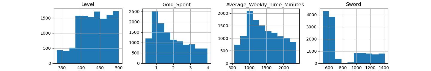
hist = csv.hist(column=['Level', 'Gold_Spent', 'Average_Weekly_Time_Minutes', 'Sword'])
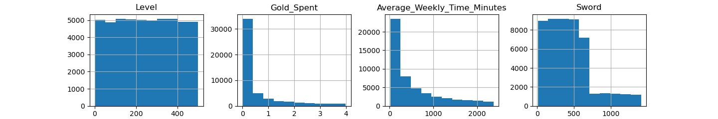
We can see that the number of samples per each bin is not equally distributed. Level is even but other values seem to follow a different distribution.
Using machine learning to cluster the players
Unsupervised learning is a category of machine learning where we don't have
specific values for the model to predict but rather we want the training phase
of the model to find similarities and generate the labels by itself. We will use
one of the simplest algorithms called K-Means. It will classify our players into
K clusters. Each cluster will have the most "similar" players. Because this is
machine learning, we can't easily predict what the clusters will be. For example
if we set K=2 we might get players segmented by their profession or just
percentiles of levels. We will try multiple values of K and see what the
results. In our Jupyter notebook we will use sklearn package to create our
first predictions and prototype. The video I recommend you to watch to learn
more is this video tutorial.
from sklearn.cluster import KMeans
kmeans = KMeans(n_clusters=2, random_state=0).fit(csv)
But it is just a single model epoch. We can test the model by predicting the cluster for all the players and adding it as a column. Then we can split the dataset into two groups and draw histograms to see what is the pattern.
csv['Cluster'] = kmeans.predict(csv)
cluster0 = csv[csv['Cluster'] == 0]
cluster1 = csv[csv['Cluster'] == 1]

cluster0.hist(column=['Level', 'Gold_Spent', 'Average_Weekly_Time_Minutes', 'Sword'])
cluster1.hist(column=['Level', 'Gold_Spent', 'Average_Weekly_Time_Minutes', 'Sword'])
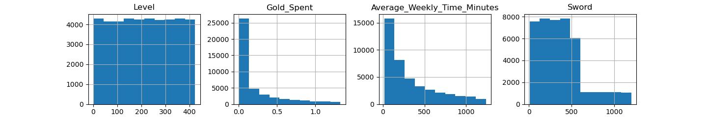
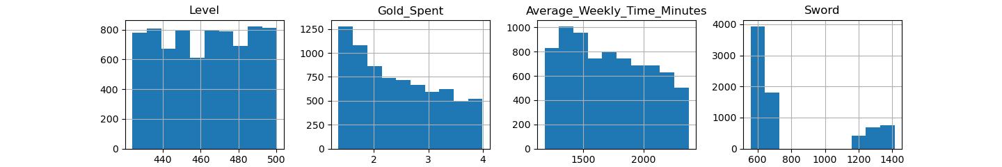
By looking at the x-axis, we can see that the players we roughly split by experience. Players with more time, gold spent and higher skills are in one cluster while the others are in the other. However, in the case of sword skill, there's a slight overlap. Let us also check if some clustering happened on one-hot profession.
print( cluster0[['Cleric', 'Wizard', 'Knight', 'Rogue']].sum() )
print( cluster1[['Cleric', 'Wizard', 'Knight', 'Rogue']].sum() )
Cleric    10703.0
Wizard    10430.0
Knight    10582.0
Rogue     10699.0
dtype: float64
Cleric    1968.0
Wizard    1903.0
Knight    1847.0
Rogue     1868.0
dtype: float64
Interestingly, the profession of the players didn't seem to matter. Why would it
be so? Well, if we simplify the K-Means algorithm to Euclidean distance between
some midpoint and vector made from each row, it would mean that level=1 has
almost the same weight as the Knight or Rogue column but when level=500,
the column doesn't matter at all. We should first scale the data to make each
column have almost the same weight (although it's not always perfect).
from sklearn.preprocessing import StandardScaler
scaler = StandardScaler()
scaled = scaler.fit_transform(csv)

kmeans = KMeans(n_clusters=2, random_state=0).fit(scaled)
csv['Cluster'] = kmeans.predict(scaled)

cluster0 = csv[csv['Cluster'] == 0]
cluster1 = csv[csv['Cluster'] == 1]

print( cluster0[['Cleric', 'Wizard', 'Knight', 'Rogue']].sum() )
print( cluster1[['Cleric', 'Wizard', 'Knight', 'Rogue']].sum() )
Cleric    9838.0
Wizard    9546.0
Knight    8392.0
Rogue     9676.0
dtype: float64
Cleric    2833.0
Wizard    2787.0
Knight    4037.0
Rogue     2891.0
dtype: float64
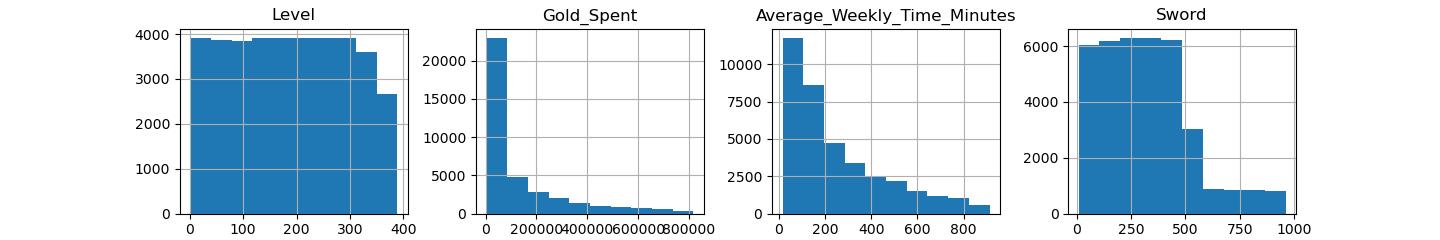
When we look at the histograms of the same columns after running K-means on the scaled dataset, we don't see that much difference in terms of clustering. The high-levels and high-spenders are still favored by the second cluster. But as you can see from the profession counts, Knights are a bit favored by the second cluster.
We can try to find the optimal number of clusters by using the elbow method where we plot the sum of squared errors (inertia) for each number of clusters.
kRange = range(2, 20)
inertias = []
for k in kRange:
    kmeans = KMeans(n_clusters=k, random_state=0).fit(scaled)
    inertias.append(kmeans.inertia_)

fig, ax = plt.pyplot.subplots()
ax.plot(kRange, inertias, '-o')
ax.axes.set_xlabel('k')
ax.axes.set_xticks(kRange)
fig.show()
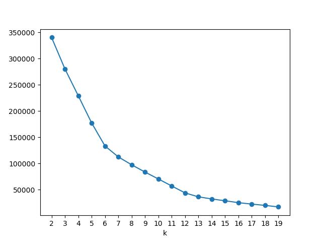
Well from this graph we can either select 6 clusters or 12 as both of them are the points where the slope changes it's direction the most. I will select 6 as it will be easier then to make a graph on how the data was clustered. We will then plot the values for some of the columns and color them by the cluster.
csv['Cluster'] = KMeans(n_clusters=6, random_state=0).fit(scaled).labels_
csv.plot.scatter(x = "Level", y = "Gold_Spent", c = "Cluster", colormap="plasma")
csv.plot.scatter(x = "Sword", y = "Magic_Level", c = "Cluster", colormap="plasma")
csv.plot.scatter(x = "Average_Weekly_Time_Minutes", y = "Gold_Spent", c = "Cluster", colormap="plasma")
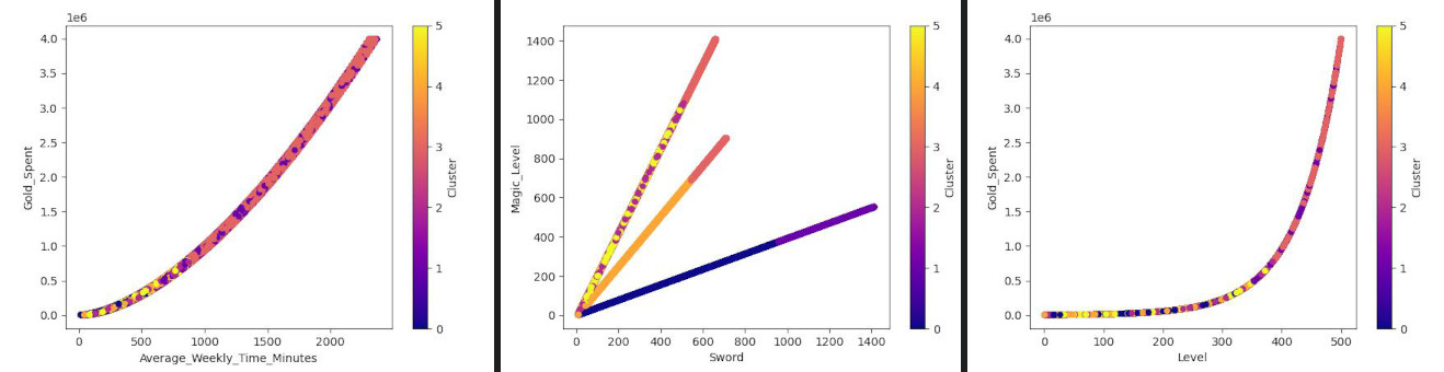
These doesn't seem to be some meaningful clusters. However, we removed the profession column in the earlier steps. Let's try to add it back and see if it helps us find any clustering.
csv['Profession'] = pd.read_csv("players.csv")['Profession']
csv.plot.scatter(x = "Profession", y = "Level", c = "Cluster", colormap="plasma")
csv.plot.scatter(x = "Profession", y = "Sword", c = "Cluster", colormap="plasma")
csv.plot.scatter(x = "Profession", y = "Magic_Level", c = "Cluster", colormap="plasma")
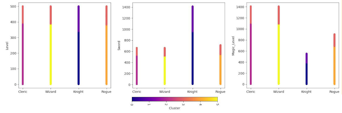
We have a clear winner here. KMeans calculated that the profession is one of the most significant lines of the split. On the graph we can see that high skilled Clerics, Wizards and Rogues are in one cluster while Knights have two clusters dedicated to themselves. All low and medium skilled players have their own distinct clusters. Because the generating script based skills, time and gold spent on the level, even including randomization, KMeans algorithm picked that up and after scaling found the correlation. However, one-hot encoding of professions make it a hard border between the data points.
Running on SageMaker
But as this is AWS exam that is coming up for me, we will run the same code on AWS SageMaker - a platform for all things Machine Learning. To do that easily, we will use SageMaker Notebooks running in AWS. To construct our infrastructure easily and destroy it afterwards to not pay too much, we will use Terraform.
If we want the notebook to be able to access our dataset, spawn SageMaker jobs
and so on, we need a proper IAM role. AWS offers us a quite permissive policy
for SageMaker that can for example access all S3 buckets which names start with
sagemaker-*. We will use Terraform to create the role and attach this policy.
resource "aws_iam_role" "sagemaker" {
    name = "SageMakerNotebookRole"
    assume_role_policy = jsonencode({
        Version = "2012-10-17"
        Statement = [ {
            Action = "sts:AssumeRole"
            Effect = "Allow"
            Principal = { Service = "sagemaker.amazonaws.com" }
        } ]
    })
}

resource "aws_iam_role_policy_attachment" "sagemaker" {
    role = aws_iam_role.sagemaker.name
    policy_arn = "arn:aws:iam::aws:policy/AmazonSageMakerFullAccess"
}
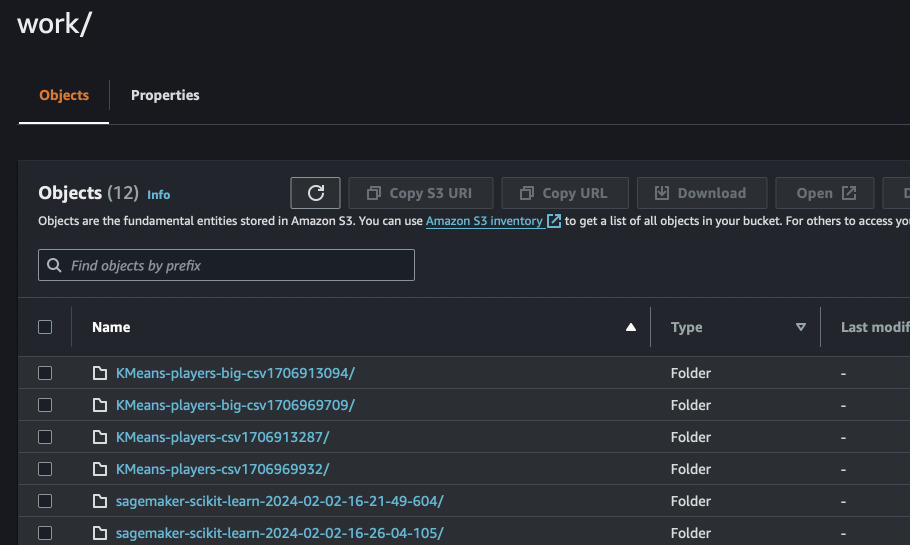
Next we will create an S3 bucket where we will upload our dataset and the actual
notebook. For the test we will generate two dataset versions: one smaller to
test Python code later inside the notebook and a larger one that will be used on
the actual SageMaker instances. Modify the script from the beginning of this
post to create a bigger dataset of 2_000_000 players. The smaller dataset we
already have will be used for testing the code inside the notebook. Change the
bucket name to something random enough but include sagemaker in the name.
Upload both datasets to the bucket (you can also do it with AWS Console).
resource "aws_s3_bucket" "sagemaker-data" {
    bucket = "sagemaker-data-2024-02-10-xyz345"
}
aws s3 cp players.csv s3://sagemaker-data-2024-02-10-xyz345/kmeans/players.csv
aws s3 cp players-big.csv s3://sagemaker-data-2024-02-10-xyz345/kmeans/players-big.csv
It's time to create a notebook. The easiest would be to create an Internet facing notebook instance. It's not as scary as you need a token either way to log in there. However, the role for this notebook will be very permissive so be sure to destroy everything after playing. We will also provide the root access to the instance so that it's easy to install some Linux packages if they are missing.
resource "aws_sagemaker_notebook_instance" "SageMakerNotebook" {
  role_arn               = aws_iam_role.sagemaker.arn
  instance_type          = "ml.t3.medium"
  name                   = "SageMakerNotebook"
  direct_internet_access = "Enabled"
  root_access            = "Enabled"
}

output "Jupyter" {
  value = "https://${aws_sagemaker_notebook_instance.SageMakerNotebook.url}"
}
You have two possibilities now to access the notebook. Either you log in to AWS
Console and use the output value Jupyter by pasting it into the browser or you
can generate a presigned URL with AWS CLI without touching AWS Console. You have
to copy this very long URL into your browser window.
aws sagemaker create-presigned-notebook-instance-url\
 --notebook-instance-name SageMakerNotebook\
 --region us-east-2\
 --query AuthorizedUrl\
 --output text
If we want to run it on SageMaker, we need an actual Python script. I converted the above notebook cells into full-length Python to be compatible with AWS and S3.
Before we can actually run our KMeans script, we need to prepare the data. We can do this in the script itself, in the notebook, but for the sake of using SageMaker, we will also post a job that will do the data preparation for us. The only thing we need is to convert Professions to one-hot encoding and perform scaling. The output we will store in the same S3 bucket.
The code is available here on GitHub. Download it, upload to your notebook instance. From there you will be able to schedule it on SageMaker instances.
First, we will create a SageMaker session. Then we will run SKLean processor
from SageMaker to run a processing job. The list of framework versions is
available
here in AWS docs.
We will put it into a function so that we can easily run it with different
parameters. First we will test if the script even works on the local notebook
instance. Then we can run the larger file on a bigger, remote instance. This
code is supposed to go into the notebook on SageMaker. Also upload
prepare-kmeans.py
to Jupyter local filesystem.
The script will also save the scaler weights that will be used later for scaling the input data during inference. For simplicity, we will use the same place as we store our processed data.
import sagemaker
from sagemaker.sklearn.processing import SKLearnProcessor
from sagemaker.processing import ProcessingInput, ProcessingOutput

BUCKET = "sagemaker-data-2024-02-10-xyz345"
sess = sagemaker.Session(
    default_bucket=BUCKET,
    default_bucket_prefix="work"
)
role = sagemaker.get_execution_role()

def process(instance_type, file_name):
    preprocessor = SKLearnProcessor(
        role=role,
        framework_version="1.2-1",
        instance_type=instance_type,
        instance_count=1,
        sagemaker_session=sess,
        env={"SM_PROCESS_FILE": file_name}
    )

    inputs = [ProcessingInput(
        source=f"s3://{BUCKET}/kmeans/{file_name}",
        destination='/opt/ml/processing/input'
    )]

    outputs = [ProcessingOutput(
        source='/opt/ml/processing/output',
        destination=f"s3://{BUCKET}/kmeans/processed"
    )]

    preprocessor.run(
        code='prepare-kmeans.py',
        inputs=inputs,
        outputs=outputs
    )

process("local", "players.csv")
## Line below will use more resources
process("ml.t3.xlarge", "players-big.csv")
If the job is successful (you see exited with code 0 and Job Complete), you
can check if the file really is in the S3 bucket. Directly in the notebook
issue command:
!aws s3 ls s3://sagemaker-data-2024-02-10-xyz345/kmeans/processed/
If everything is fine, the file should be here.
2024-02-01 19:19:31 10467734 players.csv
So we can now preview it, also directly in the notebook to verify if the job did
the thing correctly. Copy the file with another shell command in the notebook
and head() with pandas.
!aws s3 cp s3://sagemaker-data-2024-02-10-xyz345/kmeans/processed/players.csv .
import pandas as pd
pd.read_csv('players.csv').head()
     Level      Sword       Shield      Magic_Level Average_Weekly_Time_Minutes Gold_Spent  Cleric      Knight      Rogue       Wizard      Profession
0    -1.512848  -1.244164   -1.310136   -1.182956   -0.830235                   -0.620895   1.725059    -0.582215   -0.576149   -0.571346   Cleric
1    0.103096   -0.269317   -0.389385   0.578072    -0.368809                   -0.470166   1.725059    -0.582215   -0.576149   -0.571346   Cleric
2    -1.561188  -1.162927   -1.225608   -1.362817   -0.843856                   -0.621319   -0.579690   1.717577    -0.576149   -0.571346   Knight
3    -1.533565  -1.266910   -1.334287   -1.201747   -0.854072                   -0.621140   -0.579690   -0.582215   -0.576149   1.750254    Wizard
4    -0.262908  0.546304    0.365330    -0.807127   -0.569725                   -0.553066   -0.579690   1.717577    -0.576149   -0.571346   Knight
Now as the data is cleaned, we can run it on a larger, remote instance. I used
ml.t3.large as requesting c4 or c5 failed immediately with quota limits
(absurdly ridiculous).
This will take a long time. After it finished, check if the file was also put
into S3.
!aws s3 ls s3://sagemaker-data-2024-02-10-xyz345/kmeans/processed/
2024-02-01 19:47:35  407803754 players-big.csv
2024-02-01 19:35:33   10178843 players.csv
Performing KMeans on SageMaker
So as we now know how to run a processing job on SageMaker, another thing would
be to run a training job. We will run the same KMeans code in the same way as we
did with the processing job. Upload the script to the notebook instance and
create a new function that will perform KMeans training on the processed data.
The output will be a model which we will later use for inference.
Download
fit-kmeans.py from here.
Upload it to the notebook instance.
from sagemaker.sklearn.estimator import SKLearn
from sagemaker.inputs import TrainingInput
from pathlib import Path
import re
from datetime import datetime

def basename(f):
    return Path(f).stem

def train(instance_type, file_name):
    est = SKLearn(
        entry_point="fit-kmeans.py",
        role=role,
        framework_version="1.2-1",
        instance_type=instance_type,
        instance_count=1,
        sagemaker_session=sess,
        environment={
            "SM_INPUT_DATA_FILE": file_name,
            "SM_MODEL_FILE": basename(file_name) + ".joblib"
        },
        # If you happen to do some code experiments and need to test around
        # keep this line. This will charge you extra 6 minutes of instance but
        # the benefit of not needing to wait for all the downloads outweighs it.
        # Unless you get: "Instances not retained as a result of warmpool resource limits being exceeded."
        # Ask AWS support to increase the warmpool limit.
        # Amazon needs to invest better lol.
        keep_alive_period_in_seconds=360
    )

    # Regex, replace all non-alphanumeric characters with a hyphen and remove underscore duplicates.
    # And unfortunately the job has to have unique name so you have to somehow remember what you trained.
    job_name = "KMeans-" + re.sub("\\-+", "-", re.sub(r'\W+', '-', file_name)) + str(int(datetime.now().timestamp()))

    # The inputs have to be a prefix in the S3 bucket. It will be all copied over.
    # The specific file to use is specified in the environment variable.
    inputs = {
        "train":
            TrainingInput(f"s3://{BUCKET}/kmeans/processed")
    }

    est.fit(inputs, job_name=job_name)
    return est

estimator = process("ml.m5.xlarge", "players-big.csv")
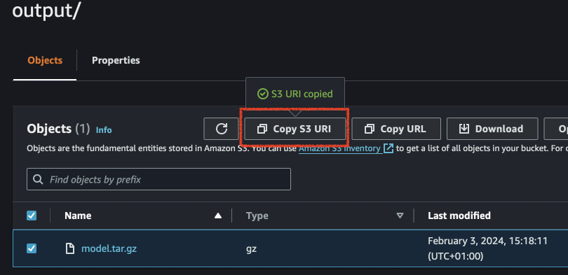
We can now check if the model was created and stored in S3.
!aws s3 ls s3://sagemaker-data-2024-02-10-xyz345/work/
    PRE KMeans-players-big-csv/
    PRE KMeans-players-csv/
The actual model file (joblib) is under
s3://sagemaker-data-2024-02-10-xyz345/work/KMeans-players-big-csv/output/model.tar.gz.
We can later refer to it in the inference script. Although the train function
above returns the actual estimator that can be also used directly for inference
after training, we will train model loading now.
Running KMeans inference on SageMaker
We have to make another script similar to kmeans-fit.py. However, this time
the script must follow SageMaker structure. We have to create model_fn
function that will be used to load the model from the S3 bucket. Then input_fn
is used for deserializing the input data (such as JSON) into the format that our
model requires. predict_fn is the function that will be called for each
prediction. It will use the model and the input data to make the prediction. As
the last step, output_fn will serialize the prediction into the format that
the caller requests. The ready file is available
here on GitHub.
In order to use the model, we have to specify the location of the tar.gz file
we got from training. I found mine in the S3 bucket we specified earlier in the
latest directory. Copy S3 URI and paste for model_data parameter.
from sagemaker.sklearn.model import SKLearnModel
model = SKLearnModel(
model_data=f"s3://{BUCKET}/work/KMeans-players-big-csv1706969709/output/model.tar.gz",
role=role,
entry_point="predict-kmeans.py",
framework_version="1.2-1",
env={"SM_MODEL_FILE": "players-big.joblib"}
)
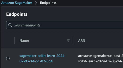
endpoint = model.deploy(
instance_type="ml.c4.xlarge",
initial_instance_count=1,
container_startup_health_check_timeout=240
)
The above lines will automatically create a model, endpoint configuration and an
inference endpoint for us in SageMaker. Upon endpoint deletion, the model record
and configuration will persist. Despite we gave an absolute path when creating
the model, SageMaker also automatically picked up which training job created
this artifact and linked the two together. If provisioning of the endpoint takes
too long, better check CloudWatch log group named after the endpoint for any
possible errors. SageMaker will retry to deploy the model a lot of times before
giving up. Hence we set the container_startup_health_check_timeout to some
small value to speed up possible failure. See
this conversation
for some hacks that didn't work for me. So far in February 2024, the default
timeout seems to be more or less 20 minutes.
After you are done with the experiments and inferences, remember to delete the endpoint or you will pay for the running instance.
# Run this AFTER you did everything.
endpoint.delete_endpoint() # Also doable via AWS Console and CLI
Because we used header names when training the model, we have to use our own method for loading CSV data. Hence we just pass the input as string and let the endpoint script parse it. The response should be JSON as we requested.
from sagemaker.deserializers import JSONDeserializer
from sagemaker.serializers import CSVSerializer
from sagemaker.base_serializers import StringSerializer

endpoint.ContentType = "text/csv"
endpoint.deserializer = JSONDeserializer()
endpoint.serializer = StringSerializer(content_type='text/csv')

response = endpoint.predict(
"""Level,Profession,Sword,Shield,Magic_Level,Average_Weekly_Time_Minutes,Gold_Spent
233,Rogue,338,522,421,246,88030
35,Wizard,54,54,102,71,5267
52,Rogue,81,127,97,90,6634
434,Cleric,571,577,1223,1336,1555266
186,Wizard,249,251,524,181,44998
"""
)
The response will be simple array with [{"Cluster": 2}, {"Cluster": 2}, ...]
for each row we sent. You can convert it to DataFrame and combine with what you
sent. Remember to delete the endpoint now if you have finished experimenting.
Predicting gold spent with XGBoost
XGBoost is an amazing tree-based algorithm but better. It isn't random like Random Forest and not a single tree. It improves with each iteration by correcting errors of the previous iteration. We will use Amazon's provided XGBoost that will train automatically on SageMaker by just providing the data.
However, we need to first prepare this data. We will use modified version of our
previous prepare-kmeans.py script to also split the data for train, test and
validation. Upload the following file to the notebook work directory:
prepare-xgb.py
And next we will create a new function for running this processor.
def processXGB(instance_type, file_name, enable_scaler=False):
    env = {"SM_PROCESS_FILE": file_name}
    destination = f"s3://{BUCKET}/xgb/{basename(file_name)}-split"

    if enable_scaler:
        env["SM_SCALER_ENABLE"] = "1"
        destination = f"s3://{BUCKET}/xgb/{basename(file_name)}-split-scaled"

    preprocessor = SKLearnProcessor(
        role=role,
        framework_version="1.2-1",
        instance_type=instance_type,
        instance_count=1,
        sagemaker_session=sess,
        env=env
    )

    inputs = [ProcessingInput(
        source=f"s3://{BUCKET}/kmeans/{file_name}",
        destination='/opt/ml/processing/input'
    )]

    outputs = [ProcessingOutput(
        source='/opt/ml/processing/output',
        destination=destination
    )]

    preprocessor.run(
        code='prepare-xgb.py',
        inputs=inputs,
        outputs=outputs
    )
We can test this function with smaller dataset on the local notebook processor. If this succeeds, we can run it on more datasets and turn on the scaler to see if the model is better with or without scaling.
processXGB("local", "players.csv")
processXGB("ml.t3.xlarge", "players-big.csv")
processXGB("ml.t3.xlarge", "players-big.csv", True)
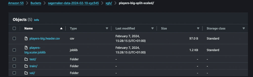
The datasets should land in our S3 bucket. We can now train the model. I will
try to do some experiments with loss function used by XGBoost to check which one
performs the best on the training split. I also included wait parameter so
that all models can be trained in parallel.
from sagemaker.estimator import Estimator
from sagemaker.image_uris import retrieve
from sagemaker.inputs import TrainingInput
import re
from datetime import datetime

def train(instance_type, prefix, loss_type="squaredlogerror", rounds=25, wait=True):
    # Last part after slash and convert all non-alphanumeric characters to hyphen
    name = re.sub("\\-+", "-", re.sub(r'\W+', '-', prefix.split('/')[-1]))
    # Add number of rounds, loss type and some timestamp to the name
    name = f"{name}-{rounds}-{loss_type}-{str(int(datetime.now().timestamp()))[-6:]}"
    # Shorten the name
    name = re.sub("square", "sq", re.sub("error", "e", name))

    xgb = sagemaker.estimator.Estimator(
        retrieve("xgboost", sess.boto_region_name, "1.7-1"),
        role,
        instance_count=1,
        instance_type=instance_type,
        output_path=f"s3://{BUCKET}/output/{prefix}",
        sagemaker_session=sess
    )

    # Large depth, eta, gamma and weight seem to work better on this dataset
    # but it overfits around 20th iteration.
    xgb.set_hyperparameters(
        max_depth=80,
        eta=0.475,
        gamma=2.5,
        min_child_weight=24,
        subsample=0.8,
        verbosity=0,
        objective=f"reg:{loss_type}",
        num_round=rounds
    )

    xgb.fit({
            "train": TrainingInput( s3_data=f"s3://{BUCKET}/{prefix}/train", content_type="csv" ),
            "validation": TrainingInput( s3_data=f"s3://{BUCKET}/{prefix}/val", content_type="csv" )
        },
        job_name=name,
        wait=wait
    )

    return xgb
We can now train the models. I will do all of them in parallel. You can observe the results in the console. On this size of the dataset, the training shouldn't take too long, 3~5 minutes.
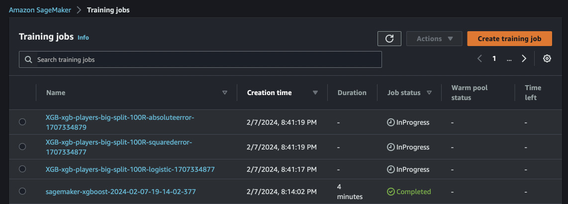
xgb_sqlog = train("ml.m5.xlarge", "xgb/players-big-split", wait = False)
xgb_sq = train("ml.m5.xlarge", "xgb/players-big-split", "squarederror", wait = False)
xgb_abs = train("ml.m5.xlarge", "xgb/players-big-split", "absoluteerror", wait = True)
# Wait here for the above to finish
xgb_sqlog_sc = train("ml.m5.xlarge", "xgb/players-big-split-scaled", wait = False)
xgb_sq_sc = train("ml.m5.xlarge", "xgb/players-big-split-scaled", "squarederror", wait = False)
xgb_abs_sc = train("ml.m5.xlarge", "xgb/players-big-split-scaled", "absoluteerror", wait = True)
Now we can evaluate the models. We will submit our testing split to the endpoint which will be copied over to the notebook instance. As it's a small subset we can safely manipulate it in the notebook. The function will spin up an endpoint from the trained evaluator, do predictions, delete endpoint and return mean square error and R-squared score.
from sagemaker.serializers import CSVSerializer
import numpy as np
import pandas as pd
from sklearn.metrics import mean_squared_error, r2_score

def evaluate(model, instance_type, data):
    pred = model.deploy(
        initial_instance_count=1,
        instance_type=instance_type,
        serializer=CSVSerializer()
    )

    actual = data.to_numpy()[:, 0]
    data = data.to_numpy()[:, 1:] # Skip first column and make it numeric
    split_array = np.array_split(data, int(data.shape[0] / float(100) + 1))
    predictions = ""
    for array in split_array:
        predictions = "".join([predictions, pred.predict(array).decode("utf-8")])

    pred.delete_endpoint()

    predictions = predictions.split("\n")[:-1]
    predictions = np.array([float(x) for x in predictions])

    for p in range(5):
        print(f"{p} (predicted, actual) = {predictions[p]:.3f}, {actual[p]:.3f}")

    return (mean_squared_error(actual, predictions), r2_score(actual, predictions))

!aws s3 cp s3://sagemaker-data-2024-02-10-xyz345/xgb/players-big-split/test/players-big.testing.csv testing.csv
!aws s3 cp s3://sagemaker-data-2024-02-10-xyz345/xgb/players-big-split-scaled/test/players-big.testing.csv testing-sc.csv
testing = pd.read_csv('testing.csv')
testing_sc = pd.read_csv('testing-sc.csv')
As the first experiment, I looked mostly at the squarederror model (second
one) and it showed some overfitting around 20th epoch. Despite the fact, I
decided to measure it against the test set. And the predictions were pretty
accurate.
0 (predicted, actual) = 352036.250, 351934.000
1 (predicted, actual) = 31445.012, 31469.000
2 (predicted, actual) = 67149.734, 67084.000
3 (predicted, actual) = 219671.359, 219695.000
4 (predicted, actual) = 17301.877, 17374.000
MSE: 3948.7184, R2: 1.0000
Let's try with other models and scaled data.
mse, r2 = evaluate(xgb_sqlog, "ml.m5.large", testing)
print(f"Squaredlog: MSE: {mse:.4f}, R2: {r2:.4f}")
mse, r2 = = evaluate(xgb_sq, "ml.m5.large", testing)
print(f"Squared: MSE: {mse:.4f}, R2: {r2:.4f}")
mse, r2 = = evaluate(xgb_abs, "ml.m5.large", testing)
print(f"Absolute: MSE: {mse:.4f}, R2: {r2:.4f}")
mse, r2 = = evaluate(xgb_sqlog_sc, "ml.m5.large", testing_sc)
print(f"Squaredlog Scaled: MSE: {mse:.4f}, R2: {r2:.4f}")
mse, r2 = = evaluate(xgb_sq_sc, "ml.m5.large", testing_sc)
print(f"Squared Scaled: MSE: {mse:.4f}, R2: {r2:.4f}")
mse, r2 = = evaluate(xgb_abs_sc, "ml.m5.large", testing_sc)
print(f"Absolute Scaled: MSE: {mse:.4f}, R2: {r2:.4f}")
The results prove that squarederror loss function performs the best (and the
only one reasonably) for the dataset in both scaled and raw versions. This can
be due to hyperparameters we selected. Either way, for a model that predicts how
much gold will a player spend based on their statistics is good enough.
0 (predicted, actual) = 617.065, 351934.000
1 (predicted, actual) = 528.865, 31469.000
2 (predicted, actual) = 528.865, 67084.000
MSE: 1127183191751.4749, R2: -0.3847

0 (predicted, actual) = 352036.250, 351934.000
1 (predicted, actual) = 31445.012, 31469.000
2 (predicted, actual) = 67149.734, 67084.000
Squared: MSE: 3948.7184, R2: 1.0000

0 (predicted, actual) = 113837.922, 351934.000
1 (predicted, actual) = 113814.094, 31469.000
2 (predicted, actual) = 113814.094, 67084.000
Absolute: MSE: 1013288335448.9435, R2: -0.2448

0 (predicted, actual) = 617.065, 351934.000
1 (predicted, actual) = 528.865, 31469.000
2 (predicted, actual) = 528.865, 67084.000
Squaredlog Scaled: MSE: 1127183191751.4749, R2: -0.3847

0 (predicted, actual) = 352038.406, 351934.000
1 (predicted, actual) = 31466.570, 31469.000
2 (predicted, actual) = 67120.523, 67084.000
Squared Scaled: MSE: 3948.1590, R2: 1.0000

0 (predicted, actual) = 113837.922, 351934.000
1 (predicted, actual) = 113814.094, 31469.000
2 (predicted, actual) = 113814.094, 67084.000
Absolute Scaled: MSE: 1013288335448.9435, R2: -0.2448
Another task would be to find a good set of hyperparameters for the model make it even more accurate. It can be done with SageMaker Model Tuning. However, this is a task for another day.